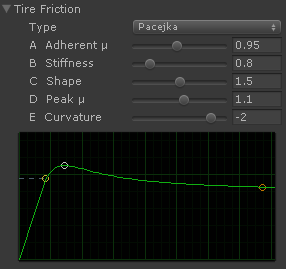
This guide explains how each parameter of the Pacejka ’94 specification affects the resulting curve, as well as their typical range of values.
The Pacejka / Magic Formula (MF) equations were conceived to fit the data gathered from experimental tests with real tires. Real Pacejka/MF data sets are heavily protected intellectual property of the tire manufacturers. However, when used in video games where gameplay is important, the Pacejka curves can be fine tuned in a variety of ways to achieve the desired result.
 Longitudinal Force

Pacejka ’94 Longitudinal Force parameters:
| Parameter | Role | Units | Typical range | Sample |
|---|---|---|---|---|
| b0 | Shape factor | 1.4 .. 1.8 | 1.5 | |
| b1 | Load influence on longitudinal friction coefficient (*1000) | 1/kN | -80 .. +80 | 0 |
| b2 | Longitudinal friction coefficient (*1000) | 900 .. 1700 | 1100 | |
| b3 | Curvature factor of stiffness/load | N/%/kN^2 | -20 .. +20 | 0 |
| b4 | Change of stiffness with slip | N/% | 100 .. 500 | 300 |
| b5 | Change of progressivity of stiffness/load | 1/kN | -1 .. +1 | 0 |
| b6 | Curvature change with load^2 | -0.1 .. +0.1 | 0 | |
| b7 | Curvature change with load | -1 .. +1 | 0 | |
| b8 | Curvature factor | -20 .. +1 | -2 | |
| b9 | Load influence on horizontal shift | %/kN | -1 .. +1 | 0 |
| b10 | Horizontal shift | % | -5 .. +5 | 0 |
| b11 | Vertical shift | N | -100 .. +100 | 0 |
| b12 | Vertical shift at load = 0 | N | -10 .. +10 | 0 |
| b13 | Curvature shift | -1 .. +1 | 0 |
Pacejka ’94 longitudinal formula
| Coefficient | Name | Parameters | Formula |
|---|---|---|---|
| C | Shape factor | b0 | C = b0 |
| D | Peak factor | b1, b2 | D = Fz · (b1·Fz + b2) |
| BCD | Stiffness | b3, b4, b5 | BCD = (b3·Fz2 + b4·Fz) · e(-b5·Fz) |
| B | Stiffness factor | BCD, C, D | B = BCD / (C·D) |
| E | Curvature factor | b6, b7, b8, b13 | E = (b6·Fz2 + b7·Fz + B8) · (1 – b13·sign(slip+H)) |
| H | Horizontal shift | b9, b10 | H = b9·Fz + b10 |
| V | Vertical shift | b11, b12 | V = b11·Fz + b12 |
| Bx1 | (composite) | Bx1 = B · (slip + H) |
F = D · sin(C · arctan(Bx1 – E · (Bx1 – arctan(Bx1)))) + V
where:
- F = longitudinal force in N (newtons)
- Fz = vertical force in kN (kilonewtons)
- slip = slip ratio in percentage (0..100)
Initial values for setting up the longitudinal curve
| Reference load | 4000 |
| Maximum load | 13000 |
| b0 | 1.5 |
| b2 | 1100 |
| b4 | 300 |
| b8 | -2 |
| all other | 0 |
Load-independent parameters
Load don’t have influence on these. If all other parameters are 0 then the curve keeps itself invariant with respect to the vertical load.
The first four (b0, b2, b4, b8) are the most relevant parameters that define the curve’s shape.
| Parameter | Typical range | Description | Related |
|---|---|---|---|
| b0 | 1.4 .. 1.8 | General shape of the curve. Defines the amount of falloff after the peak. The Pacejka model defines b0 = 1.65 for the longitudinal force. |
C |
| b2 | 900 .. 1700 | Friction coefficient at the peak (vertical coordinate) *1000. | D |
| b4 | 100 .. 500 | Peak’s horizontal position specified as “ascent rate”. | BCD |
| b8 | -20 .. +1 | Curvature at the peak. The more negative = more “sharp”. Has influence on the falloff afterwards. | E |
| b10 | -5 .. +5 | Curve’s horizontal shift | Sh |
| b11 | -100 .. +100 | Curve’s vertical shift | Sv |
| b13 | -1 .. +1 | Adjustment of the curvature at the peak. Similar to b8 | E |
Load-dependent parameters
The desired curve’s shape must be configured at the reference load. Typically the related parameters (load independent) must also be tweaked in order to conserve the shape.
These load-dependent parameters must be verified along all the load range, from minimum to maximum, in order to ensure their coherency. The coherency limit of each parameter can be located at the maximum load. The exception is b12, which must be verified at the minimum load.
| Parameter | Typical range | Description | Related |
|---|---|---|---|
| b1 | -80 .. +80 | Change of the friction coefficient at the peak. Positive = more friction with more load. Negative = less friction with more load. |
D, b2 |
| b3 | -20 .. +20 | Change of the peak’s horizontal position. Positive = increases ascent rate with load (moves to the left). Negative = decreases ascent rate with load (moves to the right). |
BCD, b4 |
| b5 | -1 .. +1 | Lineal change of the peak’s horizontal position. Similar to b3 but more lineal and with reverse effect positive-negative. Positive = decreases ascent rate with load. Negative = increases ascent rate with load. |
BCD, b4 |
| b6 | -0.1 .. +0.1 | Quadratic change of the curvature at the peak. Positive = more flat with load. Negative = sharper with load. |
E, b8 |
| b7 | -1 .. +1 | Change of the curvature at the peak. Same as b6 but more lineal. Positive = more flat with load. Negative = sharper with load. |
E, b8 |
| b9 | -1 .. +1 | Change of the horizontal shift. Positive = shifts to the left with more load. Negative = shifts to the right with more load. |
Sh, b10 |
| b12 | -10 .. +10 | Vertical shift when approaching zero load. Must be verified for coherency at the configured minimum load. |
Sv, b11 |
 Lateral Force

Pacejka ’94 Lateral Force parameters:
| Parameter | Role | Units | Typical range | Sample |
|---|---|---|---|---|
| a0 | Shape factor | 1.2 .. 18 | 1.4 | |
| a1 | Load influence on lateral friction coefficient (*1000) | 1/kN | -80 .. +80 | 0 |
| a2 | Lateral friction coefficient (*1000) | 900 .. 1700 | 1100 | |
| a3 | Change of stiffness with slip | N/deg | 500 .. 2000 | 1100 |
| a4 | Change of progressivity of stiffness / load | 1/kN | 0 .. 50 | 10 |
| a5 | Camber influence on stiffness | %/deg/100 | -0.1 .. +0.1 | 0 |
| a6 | Curvature change with load | -2 .. +2 | 0 | |
| a7 | Curvature factor | -20 .. +1 | -2 | |
| a8 | Load influence on horizontal shift | deg/kN | -1 .. +1 | 0 |
| a9 | Horizontal shift at load = 0 and camber = 0 | deg | -1 .. +1 | 0 |
| a10 | Camber influence on horizontal shift | deg/deg | -0.1 .. +0.1 | 0 |
| a11 | Vertical shift | N | -200 .. +200 | 0 |
| a12 | Vertical shift at load = 0 | N | -10 .. +10 | 0 |
| a13 | Camber influence on vertical shift, load dependent | N/deg/kN | -10 .. +10 | 0 |
| a14 | Camber influence on vertical shift | N/deg | -15 .. +15 | 0 |
| a15 | Camber influence on lateral friction coefficient | 1/deg | -0.01 .. +0.01 | 0 |
| a16 | Curvature change with camber | -0.1 .. +0.1 | 0 | |
| a17 | Curvature shift | -1 .. +1 | 0 |
Pacejka ’94 lateral formula
| Coefficient | Name | Parameters | Formula |
|---|---|---|---|
| C | Shape factor | a0 | C = a0 |
| D | Peak factor | a1, a2, a15 | D = Fz · (a1·Fz + a2) · (1 – a15·γ2) |
| BCD | Stiffness | a3, a4, a5 | BCD = a3 · sin(atan(Fz / a4) · 2) · (1 – a5·|γ|) |
| B | Stiffness factor | BCD, C, D | B = BCD / (C·D) |
| E | Curvature factor | a6, a7, a16, a17 | E = (a6·Fz + a7) · (1 – (a16·γ + a17)·sign(slip+H)) |
| H | Horizontal shift | a8, a9, a10 | H = a8·Fz + a9 + a10·γ |
| V | Vertical shift | a11, a12, a13, a14 | V = a11·Fz + a12 + (a13·Fz + a14)·γ·Fz |
| Bx1 | (composite) | Bx1 = B · (slip + H) |
F = D · sin(C · arctan(Bx1 – E · (Bx1 – arctan(Bx1)))) + V
where:
- F = lateral force in N (newtons)
- Fz = vertical force in kN (kilonewtons)
- slip = slip angle in degrees
- γ = camber angle in degrees
Initial values for setting up the lateral curve
| Reference load | 4000 |
| Maximum load | 13000 |
| Camber | 0 |
| a0 | 1.4 |
| a2 | 1100 |
| a3 | 1100 |
| a4 | 10 |
| a7 | -2 |
| all other | 0 |
Curve’s shape and horizontal behavior with load
The curve’s shape itself always depend on load at the horizontal axis according to the parameters a3 and a4.
| Parameter | Typical range | Description | Related |
|---|---|---|---|
| a0 | 1.2 .. 1.8 | General shape of the curve. Defines the amount of falloff after the peak. The Pacejka model defines a0 = 1.3 for the lateral force. |
C |
| a2 | 900 .. 1700 | Friction coefficient at the peak (vertical coordinate) *1000. | D |
| a3* | 500 .. 2000 | Peak’s horizontal position at the reference load, specified as “ascent rate”. | BCD |
| a4* | 0 .. 50 | Change of the peak’s horizontal position with load. Smaller value = bigger change with load. | BCD |
| a7 | -20 .. +1 | Curvature at the peak. The more negative = more “sharp”. Has influence on the falloff afterwards. | E |
| a9 | -1 .. +1 | Curve’s horizontal shift | Sh |
| a11 | -200 .. +200 | Curve’s vertical shift | Sv |
| a17 | -1 .. +1 | Adjustment of the curvature at the peak. Similar to a7. | E |
* Configure the horizontal behavior with load
Load-dependent parameters
The desired curve’s shape must be configured at the reference load. Typically the related parameters (load independent) must also be tweaked in order to keep the shape.
These load-dependent parameters must be verified along all the load range, from minimum to maximum, in order to ensure their coherency. The coherency limit of each parameter can be located at the maximum load. The exception is a12, which must be verified at the minimum load.
| Parameter | Typical range | Description | Related |
|---|---|---|---|
| a1 | -80 .. +80 | Change of the friction coefficient at the peak. Positive = more friction with more load. Negative = less friction with more load. |
D, a2 |
| a6 | -2 .. +2 | Change of the curvature at the peak. Positive = more flat with load. Negative = sharper with load. |
E, a7 |
| a8 | -1 .. +1 | Change of the horizontal shift. Positive = shifts to the left with more load. Negative = shifts to the right with more load. |
Sh, a9 |
| a12 | -10 .. +10 | Vertical shift when approaching zero load. Must be verified for coherency at the configured minimum load. |
Sv, a11 |
Camber-dependent parameters
They must ve verified along all the camber range in order to ensure their coherency. The coherency limit of each parameter can be located at the limits of the camber range. These parameters don’t have effect if camber is 0.
| Parameter | Typical range | Description | Related |
|---|---|---|---|
| a5 | -0.1 .. +0.1 | Change of the peak’s horizontal position. Positive = decreases ascent rate with camber (moves to the right). Negative = increases ascent rate with load (moves to the left). |
BCD, a3 |
| a10 | -0.1 .. +0.1 | Change of the horizontal shift. Same sign as camber = shifts to the left. Opposite sign as camber = shifts to the right. |
Sh, a9 |
| a13 | -10 .. +10 | Change of the vertical shift according to camber and load. Same sign as camber = shifts upwards. Opposite sign as camber = shifts downwards. The more load the more camber effect. |
Sv, a11 |
| a14 | -15 .. +15 | Change of the vertical shift. Same sign as camber = shifts upwards. Opposite sign as camber = shifts downwards. |
Sv, a11 |
| a15 | -0.01 .. +0.01 | Change of the friction coefficient at the peak. Positive = less friction with camber. Negative = more friction with camber. |
D, a2 |
| a16 | -0.1 .. +0.1 | Change of the curvature at the peak. Same same sign as camber = more flat. Opposite sign as camber = sharper. |
E, a7 |
 Simplified Magic Formula with constant coefficients
This simplification uses the four dimensionless B, C, D, E coefficients only. Numerical values are based on empirical tire data. The coefficients do not depend on load, camber, or further parameters. Source
| Coefficient | Name | Typical range | Typical values for longitudinal forces | |||
|---|---|---|---|---|---|---|
| Dry tarmac | Wet tarmac | Snow | Ice | |||
| B | Stiffness | 4 .. 12 | 10 | 12 | 5 | 4 |
| C* | Shape | 1 .. 2 | 1.9 | 2.3 | 2 | 2 |
| D | Peak | 0.1 .. 1.9 | 1 | 0.82 | 0.3 | 0.1 |
| E | Curvature | -10 .. 1 | 0.97 | 1 | 1 | 1 |
F = Fz · D · sin(C · arctan(B·slip – E · (B·slip – arctan(B·slip))))
where:
- F = tire force in N (newtons)
- Fz = vertical force in N (newtons)
- slip = slip ratio in percentage (0..100, for longitudinal force) or slip angle in degrees (for lateral force)
* The Pacekja model specifies the shape as C=1.65 for the longitudinal force and C=1.3 for the lateral force.
Hi,
I am currently doing my Mechanical Engineering Honours degree and I am investigating the Magic Formula with respect to lateral forces and pure slip.
How can I determine the parameters when the lateral force vs slip angle is given?
The Magic Formula is an empirical method. The parameters are somewhat iterated so the curve fits the real data. Here is an example:
http://white-smoke.wikifoundry.com/page/Tyre+curve+fitting+and+validation
Hi Edy,
have you got any example about tractor tires?
Hi Eddy
Also doing my mech honours degree currently.
Do you have any peer-reviewed sources on this? you explain it awesomely, but my supervisor wants something peer-reviewed :/
I got the information from different sources, from the Adams user manual to Brian Beckman’s The Physics of Racing, and many other. Pacejka information was different on all of them.
My guide is a kind of “unification” of all the sources, along with my own experimentation, so the result fits coherently with all them.
Helpful eplaination for initial study
Do I have to convert the coefficients in KN to N in the calculations? For example, a3 is in deg/KN and a4 is in N, do I convert a3 to deg/N?
You must set each parameter with the units accepted by it, without considering other parameters or units.
For example, if you have a force of 8000 N but the parameter accepts kN, then you have to feed that parameter with 8.
Hi, what is the slip ratio definition for magic formula. (you know there are two definitions)
There are more than two definitions. I had found about six different definitions when I researched the topic back then. I don’t think there’s an universally correct one, but every definition fits better or not depending on the simulation model it will be used into.
More info on this topic:
https://www.edy.es/dev/2011/12/facts-and-myths-on-the-pacejka-curves/
Hi im currently working on the oversteer and understeer charateristics of a formula studnet car, i wonder if anyone knows how to use the pacejka magic formula 89/94 to plot a graph of steering angle vs lateral acceleration through matlab
I have tire data I want to get tire parameters so can you told me about any paper or reference of post to do that
Hi Eddy, I am a beginner in car dynamic field. I finished Race Car Aerodynamics Designing for Speed recently, and working on tire analysis right now. I have MATLAB code for magic formula from previous worker, but it is really hard to understand how to guess initial values of coefficients. MATLAB requires initial guess for coefficients to do non-linear regression procedure(using fitnlm function).
The tire data I have does not have most of parameter values. Is there equations to find those parameters?
Help my small brain please 🙁
@Chris The Pacejka model is empirical, that is, you adjust the coefficients so the curve fits the actual tire data as closely as possible (curve-fitting method).
Hi Edy,
Where have you taken the typical range of parameter’s values from?
Are they applicable for any kind of tyre?
Thanks.
The typical value ranges are those that work well with the Pacejka curve as tire friction, that is, those that still produce a tire-like curve.
The Pacejka formula is just a standard trigonometric formula. The values in the coefficients define the resulting curve. Some combinations of coefficients produce curves that resemble a tire friction, and some others produce totally arbitrary curves without any similarity to a tire friction curve. The typical value ranges in this article are “recommended” values in the sense that if you adhere your coefficients to these ranges, the resulting curve will resemble a tire friction.
Hey, I’ve been building a sim for uni using the simplified model, but I’m not quite sure how longitudinal forces are meant to be applied. Simply plugging in the equation and typical coefficients causes the car to shoot forwards. Any advice?
@Tobias build a model without curves first, just flat friction. Once that works, apply a curve to the friction.
Hi Edy, I really like the content you share about car simulation in the unit and in general.
I would like to know how I apply the longitudinal force, would it be in combination with the car’s tractive force?
Hi Edy, by any chance do you know the units for BCD or how to derive them?
@Laerte that’s up to each specific simulation model. Pacejka curves only return the force produced by the tire under the given conditions.
@Mansur no idea. It’s a stiffness so it might be N/”something”, where “something” is some combination of slip ratio, slip angle, load, and camber.
Hi Edy,
May I know the origin of the formula for the coefficients BCDE with parameters b or a?
Best Regard,
Tim
@Tim if you refer to the “Simplifed Magic Formula” in the article, I found it in the Mathworks documentation: https://www.mathworks.com/help/physmod/sdl/ref/tireroadinteractionmagicformula.html
Hi Edy,
I realised that you didn’t take into account the self aligning torque Mz, only ethe lateral and the longitudinal forces. I’m kind of new to the Pacejka’s Model and I’ve seen that, in almost all the sources, they only care about lat. and long. forces, but not about the vertical force. Is this because, somehow, this moment is neglgible?
Regards,
Daniel
@Daniel, lateral and longitudinal forces depend directly of the vertical force. This vertical force is fed into the formulas as Fz.
Self-alignment torque (Mz) is a different formula similar to long-lat forces but calculates the torque applied by the tire intending to align itself to the direction of the velocity. It’s typically omitted because it’s not relevant to the actual tire forces.
How do you this curve in inspector?Depending on value i guees.Thx for article<3
Hello Edy,
I want to find lateral force using the simplified formula, but the tabulated B,C,D,E values are for the longitudinal. To find the lateral, could I just multiply the longitudinal by sin(slip angle)? If not, could you point me to standard values of the coefficients for the lateral case? Much appreciated.
@Cameron The simplified formula is applicable to both longitudinal and lateral. For the lateral, just feed it with the slip angle and use some B-C-D-E values that resemble a lateral friction curve. Remember that “Pacejka/Magic Formula” is a curve-fitting method: the coefficients have no physical meaning per-se, you simply adjust them until the curve fits the data you’re aiming for.
Hi Edy,
I was wondering what the “e()” in “e(-b5·Fz)” stands for under BCD longitudinal formula.
Any help would be appreciated.
Hey Edy, I have another question. I already answered the first one.
Where do I put the initial longitudinal and lateral load values at?
will you add pacejka formulta to your project ?
Thanks Edy, this has been an invaluable resource to understand the MF models I’ve since implemented in multiple applications for FSAE.